
Chapter 4 Shiny Examples
This part introduces example Shiny apps in R and Python that will be used for hosting examples throughout the book.
Shiny apps come in many different shapes and forms. We will not be able to represent this vast diversity, but instead we introduce some apps that showcase common patterns and fit onto the pages of a printed book reasonably well.
We will use the following Shiny apps as examples, all are implemented in both R and Python:
faithful: a “Hello Shiny!” app displaying the Old Faithful geyser waiting times data as a histogram with a slider that allows to adjust the number of bins used in the histogram — this app demonstrates the very basics of reactivity, and it is very short.bananas: an app that classifies the ripeness of banana fruits based on the color composition (green, yellow, brown) — this app demonstrates a more complex use case with dependencies, and the app also relies on a machine learning model that predicts based on user input, thus it better reflects real world use cases.lbtest: an app to test load balancing when scaling Shiny apps to multiple instances.
Let’s learn about the example apps.
4.1 Old Faithful
This is the classic “Hello Shiny!” app that you can see in R by trying
shiny::runExample("01_hello"). The app displays the Old Faithful geyser
waiting times data as a histogram with a slider that allows to adjust
the number of bins used in the histogram (Fig. 4.1).
The R version of the app was originally written by the Shiny package authors
(Chang et al. 2024).
The “Hello Shiny!” in R has no dependencies other than shiny.
The Old Faithful app in Python has more requirements besides shiny,
because the Python standard library does not have the geyser data readily
available, and you need e.g. matplotlib (Hunter 2007) for the histogram.
We wrote the Python version as a mirror translation of the R version,
so that you can see the similarities and the differences.
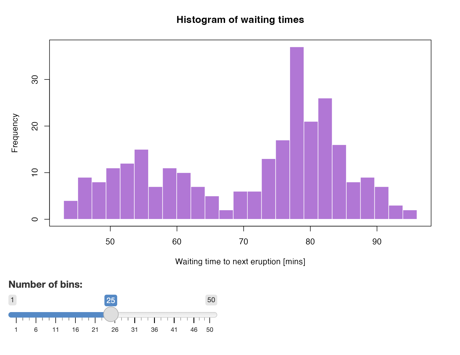
Figure 4.1: The faithful example Shiny app.
In R, the data set datasets::faithful (R Core Team 2024) contains waiting time between eruptions and
the duration of the eruption for the Old Faithful geyser in Yellowstone National
Park, Wyoming, USA. We got the Python data set from the Seaborn library
seaborn.load_dataset("geyser") (Waskom 2021).
The source code for the different builds of the Old Faithful Shiny app is at
https://github.com/h10y/faithful. You can download the GitHub repository
as a zip file from GitHub, or clone the repository with
git clone https://github.com/h10y/faithful.git.
4.2 Bananas
The bananas app was born out of a “stuck-in-the-house” COVID-19 project when
one of the authors bought some green bananas at the store and took daily
photographs of each fruit.
The Shiny app consists of a plot showing the colour composition of the ripening banana fruits (Figure 4.2). The three numeric inputs on the left hand side of the plot control the position of the red dot, which is then used to tell the ripening stage of the banana represented by the red dot.
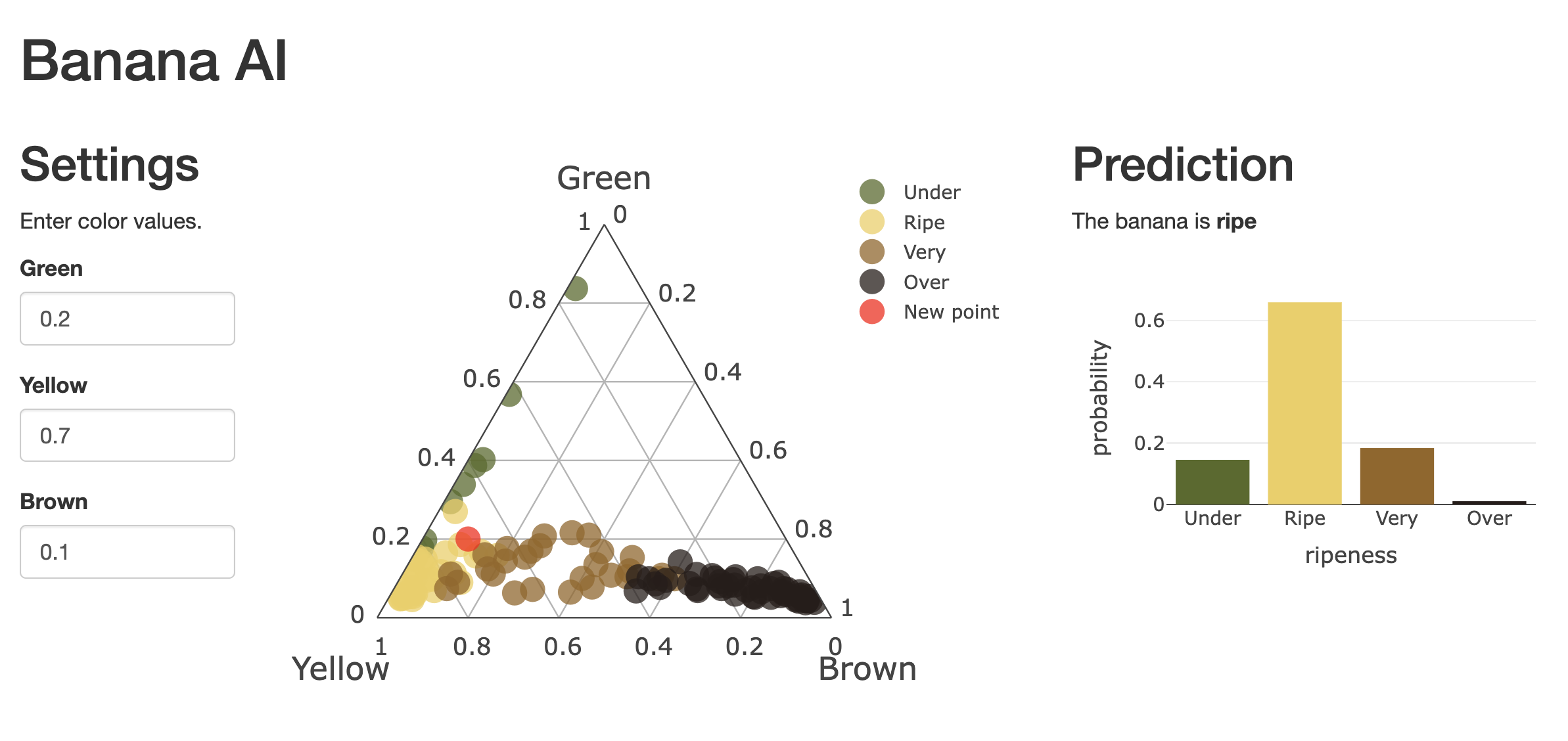
Figure 4.2: The bananas example Shiny app.
The app is more complex than the Faithful example and has more dependencies. We will use this app to illustrate the management of these dependencies during deployment and hosting.
See the Appendix for the description of the app.
The source code for the different builds of the Bananas Shiny app is at
https://github.com/h10y/bananas. You can download the GitHub repository
as a zip file from GitHub, or clone the repository with
git clone https://github.com/h10y/bananas.git.
4.3 Load Balancing Test
Shiny apps can run multiple sessions in the same app instance. A common problem when scaling the number of replicas for Shiny apps is that traffic might not be sent to the same session and thus the app might randomly fail. This app is used to determine if the HTTP requests made by the client are correctly routed back to the same R or Python process for the session.
Both the Python and the R version of the app registers a dynamic route for the client to try to connect to. The JavaScript code on the client side will repeatedly hit the dynamic route. The server will send a 200 OK status code only if the client reached the correct Shiny session, where it originally came from (Fig. 4.3).
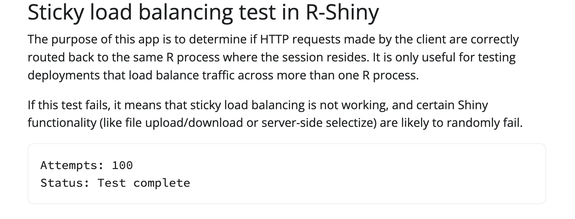
Figure 4.3: The lbtest example Shiny app.
The original Python app was written by Joe Cheng and is from the rstudio/py-shiny
GitHub repository. We wrote the R version to mirror the Python
version.
This app will be useful when the deployment includes load balancing between multiple replicas. For such deployments, session affinity (or sticky sessions) needs to be available. This app can be used to test such setups. If the test fails, it will stop before the counter reaches 100 and will say Failure! If the app succeeds 100 times, you’ll see Test complete. The app is not useful for testing a single instance deployment, or with Shinylive, because these setups won’t fail, but you can still try it.
The source code for the different builds of the load balancing test Shiny app is at
https://github.com/h10y/lbtest. You can download the GitHub repository
as a zip file from GitHub, or clone the repository with
git clone https://github.com/h10y/lbtest.git.
4.4 Summary
This is the end of Part I. We covered all the fundamentals that the rest of the book builds upon. In the next part, we’ll cover all the technical details of Shiny hosting that happens on your local machine.
We recommend downloading the example repositories mentioned in this chapter
to your computer. This way you will be able to follow all the examples
from the following chapters and won’t have to copy paste the text from the
book to files. Visit the GitHub organization h10y which stands for
hostingshiny (there are 10 letters between the first h and the last y):
https://github.com/h10y/.